Online learning with a memory-efficient Kalman Filter
Introduction: The Kalman Filter
Recently, I had the opportunity to learn about the Kalman filter: a powerful, versatile tool that captures uncertainty in a time-varying system. Given a series of observations and an underlying dynamical model of how the state should change over time, the Kalman filter can update the state based on a probability distribution of the state and external observation data. It is no surprise, then, that NASA was able to utilize these properties for many aerodynamic control systems, including the famous Apollo missions to the moon!
However, another use of the Kalman filter outside of control theory is Bayesian machine learning. Rather than traditional methods of optimizing a model, we can frame the idea of model learning in terms of uncertainty: we start off being highly uncertain that our model parameters are optimal, and ideally use a variant of the Kalman filter algorithm to shrink our uncertainty (and therefore naturally optimize the model in the state-estimation process). As it turns out, this is not only reasonable, but also quite performant; the calculations incorporate approximate second-order information${}^1$ when computing the next state. We call this method the Extended Kalman Filter (EKF).
The EKF algorithm
We can roughly describe the algorithm in the following steps:
- “A priori” predictions${}^2$; essentially, making a simple prediction of what the next EKF state will be (in our case, the model parameters). $\theta$ represents the model parameters as a vector, $\Sigma$ represents the covariance matrix of the parameters, $\mathbf{Q}$ represents the process noise, and $\mathbf{f_\theta}$ represents the output of the model with parameters $\theta$. To generalize this problem to one in control theory, let’s suppose we are learning to optimize controls over a system that has system state $\mathbf{x}$ and controls $\mathbf{u}$, and our underlying baseline model predicts an observation $\mathbf{y}$.
- Kalman gain computation, which helps scale how much to change the parameters (almost like a “learning rate”). $\mathbf{R}_t$ is the observation noise, and crucially, $\mathbf{K}_t$ is the Kalman gain matrix.
- Posterior computation, which uses the Kalman gain to update the state distribution. $\mathbf{I}$ is the identity matrix while $\mathbf{s}_t$ is the innovation: the difference between the predicted state $\mathbf{y}_{t+1 \mid t}$ and the observed state $\mathbf{y}_{t+1}$.
This process is repeated for each timestep $t$.
In practice
Using the JAX library in Python, the above algorithm can be implemented as follows:
Click to show code
import jax
import jax.numpy as jnp

# Any functions not defined can be assumed to work as the signature implies.
def ekf_step(self, mean_t, cov_t, control_t, obs_tp1):
    # A priori predictions
    mean_tp1_apriori = mean_t
    cov_tp1_apriori = cov_t + process_cov_fn(
        mean_tp1_apriori
    )
    obs_tp1_apriori = observation_fn(
        mean_tp1_apriori, control_t
    )

    # Kalman gain calculation via Jacobian
    jac_obs = jax.jacrev(observation_fn, argnums=0)(
        mean_tp1_apriori, control_t
    )
    R_t = observation_cov_fn(mean_tp1_apriori)
    S_t = jac_obs @ cov_tp1_apriori @ jac_obs.T + R_t
    kalman_gain = (
        cov_tp1_apriori @ jac_obs.T @ jnp.linalg.inv(S_t)
    )

    # Posterior calculation
    innovation = obs_tp1 - obs_tp1_apriori
    mean_tp1 = mean_tp1_apriori + kalman_gain @ innovation
    eye_cov = jnp.eye(cov_t.shape[0])
    cov_tp1 = (eye_cov - kalman_gain @ jac_obs) @ cov_tp1_apriori

    return mean_tp1, cov_tp1
The EKF works remarkably well for regression problems. We can easily frame regression as a state-estimation problem to fit the algorithm above: the output of $\mathbf{f}_\theta$ should minimize the innovation under a constant control of $\mathbf{u}_t=\vec{0}$, $\forall t$. Here, I demonstrate the results of training a simple 641-parameter multilayer perceptron${}^3$ with two hidden layers:
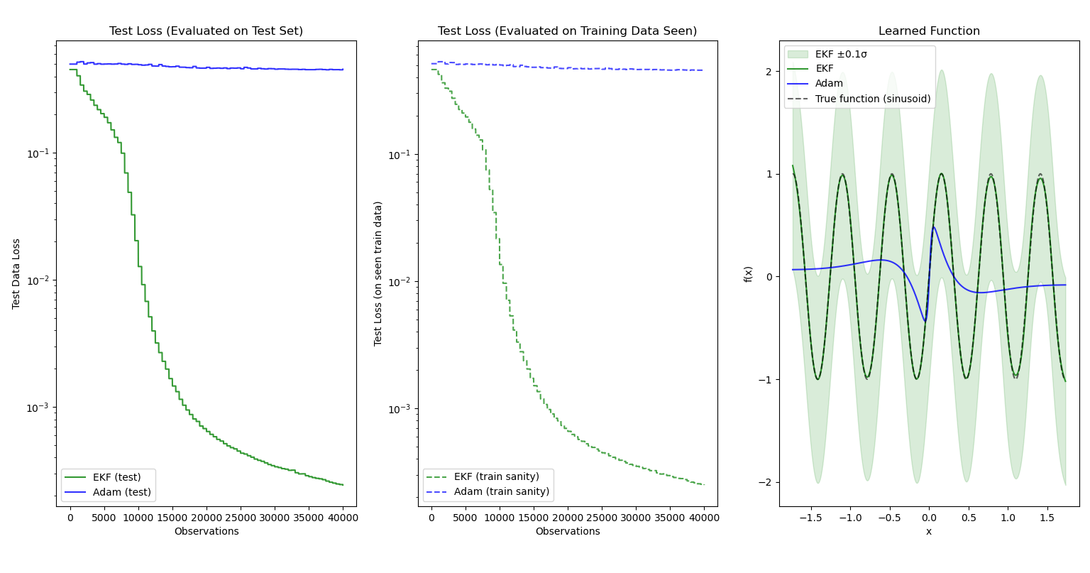
The Adam optimizer is used as a baseline. The function to be learned online is $f(x) = \text{sin}(10x)$.
As expected, the EKF performs much better than gradient-descent optimizers due to the second-order information the EKF has access to. The shaded bands around the EKF function output represent the predictive variance calculated via the following formula, $\text{Var}(y \mid x) = \textbf{S} = J_\theta \Sigma J_\theta^\top + R$ where $J_\theta = \frac{\partial \textbf{f}}{\partial \theta}(x, \theta)$, which we already calculate in the EKF algorithm.
Notice that the bands only represent $0.1$ standard deviations from the mean, signaling the scale of uncertainty. I displayed only $\pm 0.1\sigma$ to better capture the detail of the output functions, otherwise Matplotlib would have squished them to be a straight line!
Optimization: LOFI
Motivation
There is but one issue with the Kalman filter: it’s computationally and spatially expensive. The covariance matrix grows quadratically with the number of model parameters, making training large models impractical unless you have an impractical amount of RAM (and, with the current AI boom raising prices, an impractical amount of money for it). Even with large amounts of memory, the computational complexity of calculating inverses and performing the necessary matrix operations scales with the size of the covariance matrix, making training inefficient even with a GPU.
The plots I generated above required minutes of training for the EKF over the same data as Adam, which took just a few seconds. This surely wouldn’t fly in real-time systems despite their accuracy!
Using decomposition to approximate EKF
In 2023, this paper${}^4$ presented a way to approximate an EKF by storing the inverse covariance matrix in two components: a diagonal matrix and a low-rank (horizontal) matrix. Using singular value decomposition and Woodbury identities, we can still mimic the Kalman filter process of updating state distributions based on Jacobians. However, covariance updates are now much faster since the covariance information we store grows linearly with the number of parameters! We can then adjust how much covariance information we would like to capture by changing the maximum rank $L$ of the low-rank matrix.
Due to the extra complications of using covariance matrices in this format, prediction and updates are split into separate algorithms in LOFI. Moreover, while the diagonal matrix and low-rank matrices are stored independently, the update step must take care to treat them as approximating the same matrix when combined, thus any updates to one of the components must be reflected in the other. This is where SVD comes in during the update step. Still, if you look beyond the fancy matrix computations, many of the steps are similar to the standard EKF procedure: a priori predictions of parameters and the covariance matrix are the same (at least for the diagonal component), and the parameters are updated by using innovation and a modified Kalman gain matrix.
Performance
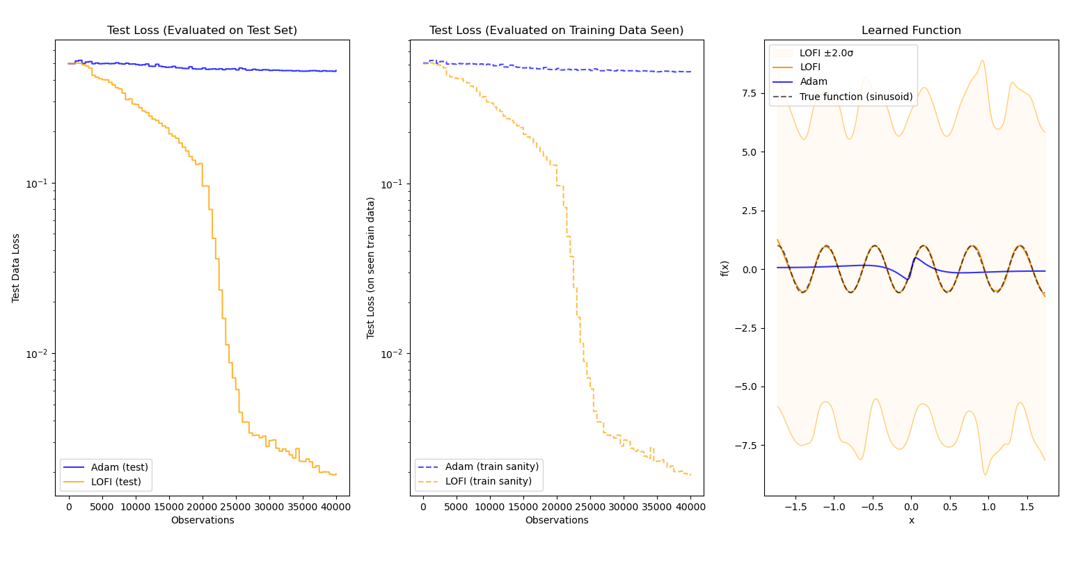
When evaluating the tradeoffs of an optimization, it’s important that the sacrifices made for speed do not lead to an optimizer that is pointlessly more complicated than a standard optimizer (i.e. does not give much performance benefit). Fortunately, this is not the case for LOFI! The following results pit LOFI${}^5$ and Adam against each other as they learn a nonlinear function online over 50,000 observations. For every 500 observations, evaluation over the test data as well as previously-seen observations is conducted and plotted.
Evaluated on $f(x)=\text{sin}(10x)$:
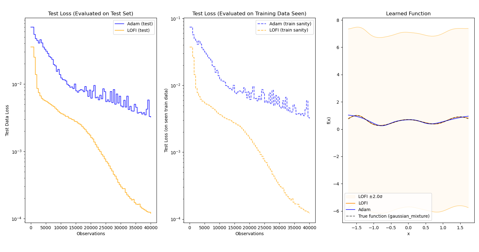
Evaluated on $f(x)=e^{\frac{-(x+1.5)^2}{0.18}} + 0.7e^{-2x^2} + 0.9e^{\frac{-(x-1.5)^2}{0.32}}$:
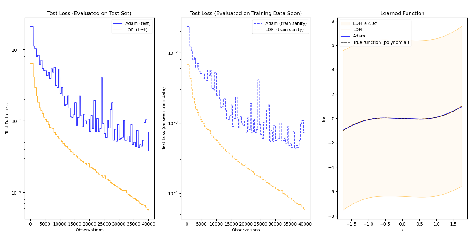
Evaluated on $f(x)=x^3-x$:
Evaluated on $f(x) = \text{sgn}(\text{sin}(10x))$ (essentially a square wave):
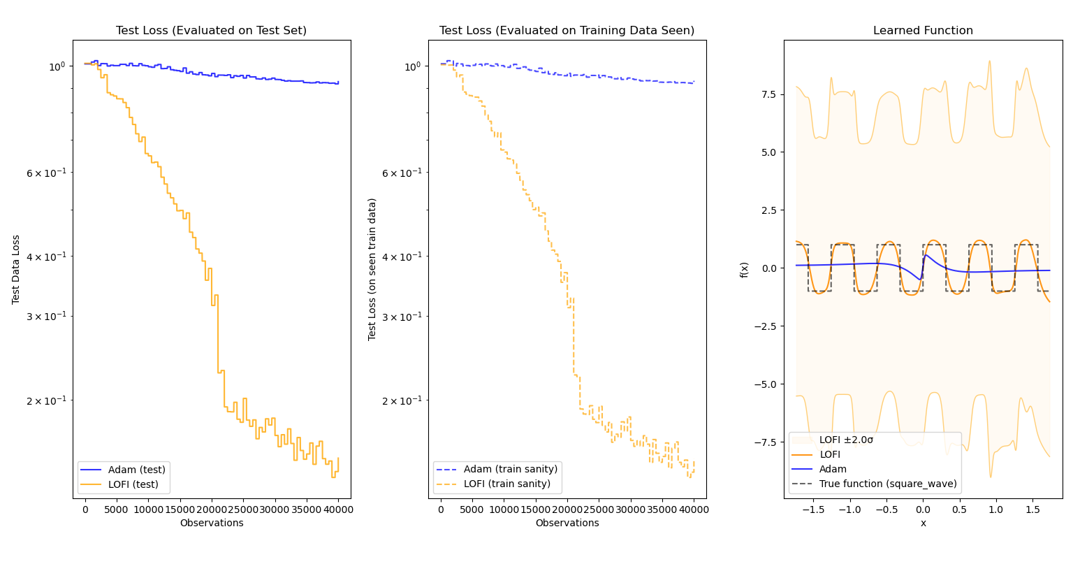
In each case, not only does LOFI approximate the function better than Adam (sometimes by a large margin), it also learns more quickly and accurately over time. More importantly, the efficiency of LOFI makes the difference in training time between the two optimizers nearly negligible.
We can also see the accuracy-for-speed tradeoff more clearly when pitting LOFI against EKF:
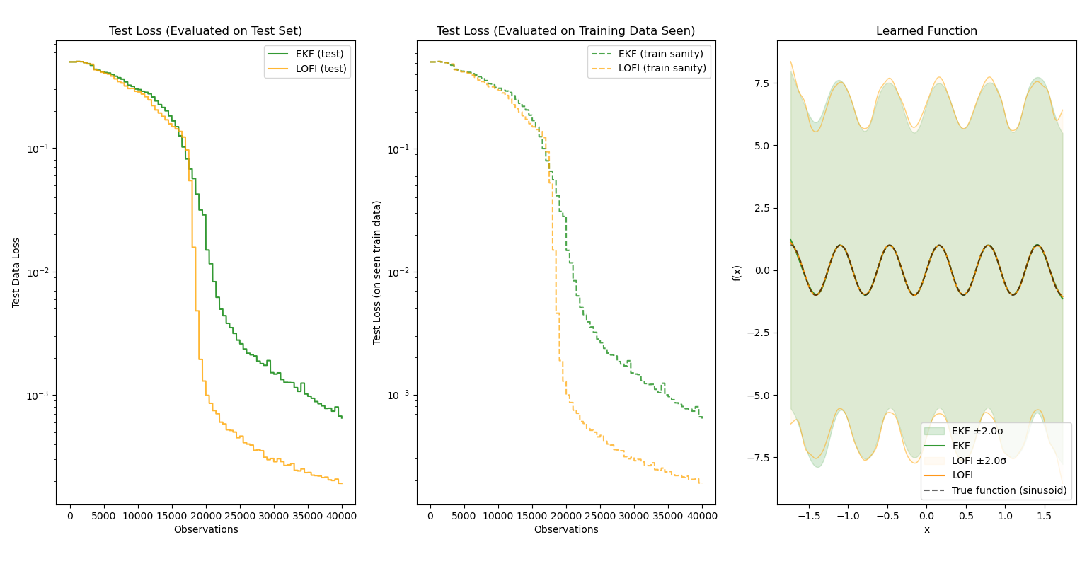
Both optimizers were able to learn the function quite well, and surprisingly, LOFI exceeds the performance of the EKF using the same shared hyperparameters${}^6$! This is likely due to implicit regularization from the low-rank approximation, as the standard EKF is more expressive than LOFI. However, observe the uncertainty bands — the EKF has slightly more certainty and its uncertainty bands match the function shape more accurately. (I suspect this is due to the low-rank approximation that LOFI uses encoding less covariance information.) Yet what is not displayed is the training time: while the EKF trained for ~3 minutes, LOFI took a mere 18 seconds to train. Given the closeness in performance, LOFI is a remarkable optimization over the EKF.
My experience with online learning
I should note that before this project, I had little experience with traditional machine learning and neural networks beyond a couple online Google Colabs that abstracted away many of the intricacies and charms of the the field, and having seen it as nothing more than a tool where the magic is already done for me, displayed little interest. But with this more technical approach to machine learning where I had to build an unconventional trainer from scratch, I realize the art of training a neural network is far from boring. Of the many things I learned, here are a few of the major points that I’ll certainly keep in mind for the future:
Normalization matters
It’s incredible how normalizing an input dataset to be centered around 0 can do wonders! While it isn’t necessary for all cases, it helps stability and convergence during training since neural nets are rather sensitive to large changes in magnitude. In fact, I found that all models were much more apt at predicting function values from inputs between [-1,1] than other input values regardless of optimizer choice.
Training is extremely sensitive to hyperparameter selection
I don’t exactly recall which paper demonstrated the role of good hyperparameter selection in convergence, but one of the featured graphs was shocking: when plotting convergence successes based on two hyperparameters only, the regions of success were completely erratic and impossible to explain! There would be small spots where the model would find a local minima amid a sea of failed convergences corresponding to bad hyperparameter pairs. Meanwhile, I had to worry about many different aspects of training for LOFI:
- What should the maximum rank $L$ of the low-rank matrix be?
- How large should the initial covariance be?
- How much process noise should I add?
- How much observation noise should I add?
I must have spent a couple hours in total trying out different combinations and increments before getting a stable model. For this, the Weights and Biases API was quite helpful in documenting past runs and making sure I didn’t waste my time with redundant runs.
JIT and vectorize EVERYTHING
In machine learning, there are a lot of repetitive calculations done inside loops on large batches of data. Thus, when doing deep learning in Python, this leads to slow, inefficient programs that simply make my laptop fan very angry for very long periods of time. Luckily, JAX also comes with several tools to make Python code quite fast by turning functions into compiled machine code with the @jax.jit decorator (the proper term for this is Just-In-Time Compilation, which you may have heard of in the context of Java). While it is quite strict with the kind of code you can have jitted, the improvements are as expected: the difference between compiled and interpreted code in terms of speed is night and day.
Additionally, because data is often handled in batches, vectorizing these operations can also lead to enormous performance enhancements. JAX’s jax.vmap and jax.lax.scan functions can modify functions to handle large amounts of data and compile slow loops into optimized machine code, respectively. These are useful when writing training scripts, as tasks like test set evaluation can easily be batched.
NaNs are really really really really annoying
Early on, the LOFI trainer would proceed fairly smoothly (albeit suboptimally) until some critical juncture of observations or epochs, after which the loss would become noticeably unstable and spike until three dreaded letters displayed to the screen:
NaN
Unlike traditional errors, it’s incredibly difficult to pinpoint the source of NaNs entering the learning pipeline, especially with so many matrix operations and inverses. Furthermore, jitting a function effectively means goodbye to any kind of effective debugging, as the Python debugger cannot follow machine code well and there was simply too much information to print.
Eventually, I implemented the following to fix the mathematical issues (as far as I’m aware of):
- Using Moore-Penrose pseudo-inverse operations for potential singular matrices
- Ensuring the returned Jacobian is a matrix to avoid dimension mismatch issues
- Adding an adaptive “jitter” value to maintain a non-zero floor for covariance (minimum 0.01)
That last modification to the algorithm was what truly helped, as the covariance would often collapse to near-zero a few observations before a NaN appeared. Maintaining mathematical stability in the algorithm enabled me to use more aggressive learning rates and thus have LOFI performance exceed that of Adam and compare to EKF.
Conclusion and Future Work
Overall, this was a valuable exploration into the world of more cutting-edge machine learning methods beyond simple gradient-descent and backprop, though I believe it would be a good idea to properly learn the fundamentals of machine learning more rigorously through my coursework and more projects like this one. Additionally, the aforementioned paper tested out LOFI learning on the MNIST dataset to test its ability to handle classification problems. Unfortunately, I was not able to set that up well, as it would take ages to train a proper-sized MLP for the job (perhaps an inefficiency with my script). I’m certainly looking forward to more work in this area, especially concerning applying such methods to non-trivial problems.
-
The EKF algorithm is a variant of the Gauss-Newton method with diminishing step size. Both methods use first-order approximations of the Hessian matrix that can solve nonlinear least-squares problems.
-
In the general EKF algorithm, the a priori predictions of state and covariance are governed by an underlying baseline model of how state changes w.r.t control (common in control theory), and will thus have extra computation not presented here. Since our state is instead the parameters of the model, the “baseline model” is simply the identity function, and thus the extra computation can be abstracted away.
-
The layers had 32 and 16 weights repectively, with $\text{tanh}(x)$ as the activation function for each layer.
-
Chang, Peter G., et al. “Low-rank extended Kalman filtering for online learning of neural networks from streaming data.” arXiv preprint arXiv:2305.19535 (2023).
- LOFI here uses the following hyperparameters:
- $L = 8$
- $\mathbf{Q}=qI$, $q=10^{-4}$
- $\mathbf{R} = \frac{1}{r}I$, $r = 10^{-1}$
- $\Sigma_0 = cI$, $c = 1.0$
- LOFI is now modified to use $L = 12$, as the paper recommends that for $L \geq 10$, LOFI performance is roughly the same as EKF. All other hyperparameters are consistent between the two and are listed above.